Transformer Details Not Described in The Paper

Since I’m a complete newbie of the deep learning field, I was looking for something to learn as a first step. Then, I heard that Transformer-based models are outperforming existing state-of-the-arts. I ignored it at first and I thought this was just a passing fad because this field changes so quickly. However, it’s still popular even though over a year has passed since the introduction. Thus, I decided to try it by myself.

Transformer is a deep learning model introduced by Attention Is All You Need at 2017. It has been actively studied in various fields nowadays. Since there is a reference code written in tensorflow (tensor2tensor) of Transformer, I could just study it by reading their paper and the implementation, but I wanted to catch all the details that I might miss, so I tried to implement it from scratch in pytorch.

At first, it was quite straightforward to implement the paper, but I noticed soon that there is some difference between my implementation and the tensor2tensor code. I found that there had been many updates since the paper was published, and there are some parts not matched with the paper. I also had a hard time to implement things not described in the paper. Now, I guess I’ve caught most of them, and I want to share what I found during the implementation. I’ll skip the clear details of Transformer written in the paper such as the architecture of Transformer. I think there are already many good sources explaining them.

I used WMT de-en dataset which is the same with translate_ende_wmt32k_rev of tensor2tensor. Each setting of max length, warmup, and batch size was 100, 16000, and 4096. Note that batch size means the number of tokens per a mini batch.

Pre/post-processing Sequence for Each Sub-Layer

I found that the order of pre/post-processing in the implementation was not like the paper. It seems like it was updated after writing the paper. The previous version of the output of each sub-layer was

but now the output is changed to

We also have to normalize the final outputs of encoder/decoder at last.

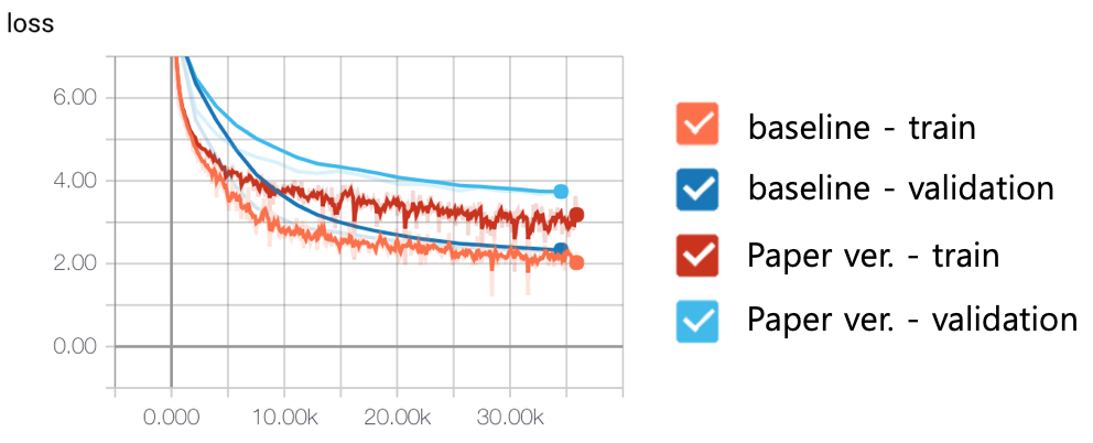
The left and right figure represent the paper version and the actual implementation. At first glance, I thought it was just switching the order, but this is actually more than that. The paper version normalizes sub-layer outputs after adding residual connections, but tensor2tensor only normalizes sub-layer inputs and don’t touch residual connections. The following figure shows the effect of this new architecture. baseline is the actual implementation in tensor2tensor and Paper ver. is the old version. As you see, this makes a huge improvement.

Fast Decoding

Transformer could achieve good quality thanks to avoiding autoregressive computations like RNN. But, unlike training steps, decoding (inference) steps still have to be autoregressive. Optimizing the decoding steps is indispensable for production.

We can optimize autoregressive steps by caching unnecessary repetitive computations. Decoding steps expand targets one by one after getting output from Transformer and feed the expanded targets until we reach the EOS token. The point here is that inputs never changes. We only have to get Encoder Output once and reuse it for the rest decoding steps, which improves decoding speed 1.33 times faster. Furthermore, the Encoder Output is used to get K and V value for encoder-decoder attention. We can also keep these values and reuse them, which makes it 1.42 times faster.

This is all I found about fast decoding, but I’m sure there are more we can optimize. For instance, we don’t need to repetitively compute positional encodings or networks for previous targets. Half of self-attention values in decoder are zeros because its attention mask shape is triangular, then we might be able to avoid computations with sparse computation techniques like blocksparse.

Data Preprocessing

The ways of feeding data influence performance of training a lot. This may be a topic for general training of NLP models, so it might be inappropriate for this post, but I want to share what I’ve learned from tensor2tensor code.

Paddings

Since NLP tasks have variable-length data, we need to add paddings to make the same size with other inputs in a mini-batch. Then, we have two problems. First, it’s a waste of resources to load and compute paddings. If we can minimize the fraction of paddings, then we can make the training much faster. In my case, when 60% of my data were paddings, it took 250 sec for each training epoch, but it became 100 sec after reducing the fraction of paddings to 5%. Second, computations for paddings could be noise. In Transformer, paddings became non-zero after passing normalization layers. This makes gradients for each padding, which makes unnecessary weight updates. I found that many other implementations are handling this issue (e.g. reset paddings to zero at every sublayer). But, surprisingly, tensor2tensor does not handle paddings in encoder/decoder layers. It just multiplies zeros to paddings in embedding layers, and ignore paddings of inputs by masking paddings in attentions.

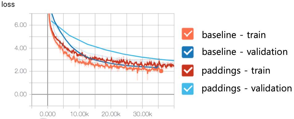
tensor2tensor focuses on reducing the fraction of paddings rather than handling paddings in the model itself. They use bucketing by sequence lengths. It is just to group sequences which have similar lengths. In the following figure, paddings is to feed data sequentially regardless of sequence lengths, and baseline is a naive implementation of tf.bucket_by_sequence_length in pytorch.

Data Sharding

tensor2tensor splits datasets into multiple shards because we cannot load all data on memory if data is too big. So, tensor2tensor iterates and loads each shard one by one for training. One important thing is that each shard has an equal distribution of datasets.

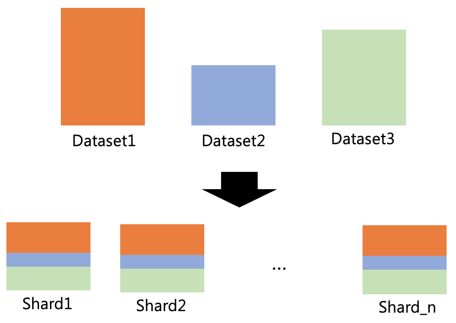
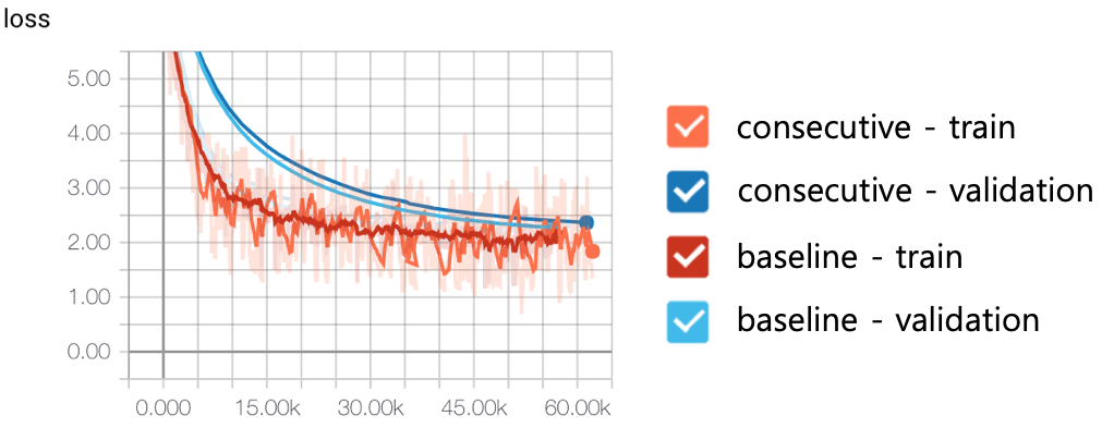
We sometimes gather datasets from multiple sources to make a “big data”. Then, each dataset may have inconsistent characteristics, so feeding them sequentially may lead to slow convergence of training. Shuffling data is one option to handle the issue, but shuffling big-data is not simple. So, tensor2tensor just makes each shard to have an equal distribution of datasets of different sources and shuffles only small fraction of entire dataset. This strategy stabilizes training like the following figure. consecutive is to feed data consecutively whose dataset is not well distributed, which shows a lot of fluctuation and slow convergence in the validation set.

Minors

Weight Initialization

As we all know, weight initialization is one of the important factors for training. Xavier (glorot) uniform initializer with \(1.0\) gain is the initializer for encoder and decoder layers. But, one more thing we should be careful about is that we have to initialize embedding layers with a random normal initializer with \(0.0\) mean and \(d_{model}^{-0.5}\) stddev settings.

Positional Encoding

Transformer has a special encoding for positional information like this:

But, the actual implementation gets positional encodings by the following formula:

I think this does not make a big difference in performance because positional encoding is just a heuristic to make a difference between relative positions, but we just need to be careful when we have to load pre-trained frozen embeddings.

Dropout

The paper described only two dropouts: one in the output of each sub-layer and the other in the embedding layers. But, two more dropouts are added to Transformer. Transformer has dropouts after ReLU in position-wise feed-forward networks, and after SoftMax in attentions.

Hyperparameter Settings

There are many updates on the default hyperparameter settings. For example, learning rate is doubled. They updated \(\beta_{2}\) of Adam optimizer to \(0.997\). The default values of warmup steps for single GPU and others are also updated to \(16000\) and \(8000\). Epsilon value for layer normalization is \(10^{-6}\).

Conclusion

Since deep learning is mostly based on empirical studies. Some researches are overfitted to a specific problem. There could be some important details authors didn’t realize, or authors may overemphasize not so critical points. Sometimes, unintended implementations make performance improvements. Thus, it’s important to try models by yourself.

Actually, I first tried to build my own neural networks instead of using well-known architectures to solve my own problem before starting this project, but it didn’t work well. Since there is no clear answer in this field, it was really hard to debug and improve it. Implementing Transformer from scratch helped me to study cases with a concrete answer. At least, I was able to move toward the reference implementation. I couldn’t still understand why those small changes make different behaviors, but this experience will help me to debug neural network models in the near future. I recommend you to implement well-known architectures from scratch.

You can find my code in https://github.com/tunz/transformer-pytorch.